How to import data into Apyesse

Once you have purchased Apyesse and obtained the setup program, the installation steps are simple and guided and do not require system skills or the installation of third-party components. This tutorial uses the demo database that can be optionally installed with Apyesse. This database (Sqlite) simulates the role of the company management system and allows the user to test the Apyesse functionality independently.

Once you launch Apyesse for the first time, the next thing you need to do is create a datastore:

• from the ‘Database’ menu choose ‘New’
• then you select the path and name of the database

Now we need data to work with. These can be imported from an external source (typically the ERP system) or, in the case of simulations, they can be created from a Python script, the language that Apyesse uses to automate tasks.

As mentioned above, in this tutorial we will use a demo database to simulate the data source consisting of the ERP and we will import data from it via an ODBC connection (for the demo database this connection is already created during the Apyesse installation wizard).

After creating the database, click on the button represented in the following figure for the guided creation of a data loading procedure in Apyesse

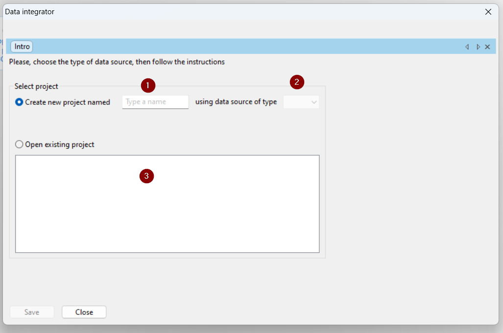
At this point the first page of a wizard opens which facilitates the creation of a procedure to feed the Apyesse database. The first step is the definition of a data exchange project, choosing a new or existing one to modify. Related to the following image:

1. if you choose to start a new integration project, you define its name
2. and you choose the type of data exchange technology to use
3. otherwise, if previous exchange projects have already been created, double click on the corresponding project

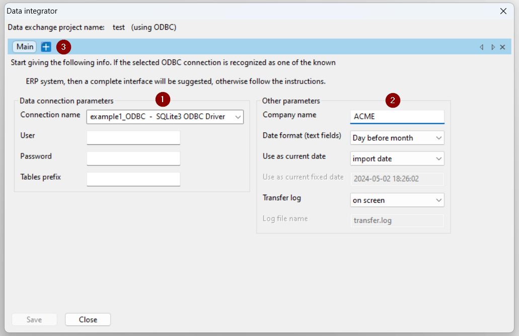
At this point, assuming we continue with the guided procedure for creating a new data exchange project, after selecting the ODBC type, the following dialog box opens, where:

1. you select from a list the ODBC connection to use to access the data you want to import into Apyesse. The connection for the demo database is already created during the installation of Apyesse, while for the database of your ERP or other databases it is necessary to set it manually using the methods provided by Windows or by choosing the last item from the list “Create new connection.. “
2. indicate the name of the company (real or hypothetical) to be associated with the data model
3. then click on ‘+’ to begin mapping the various tables between the data source database and the Apyesse database

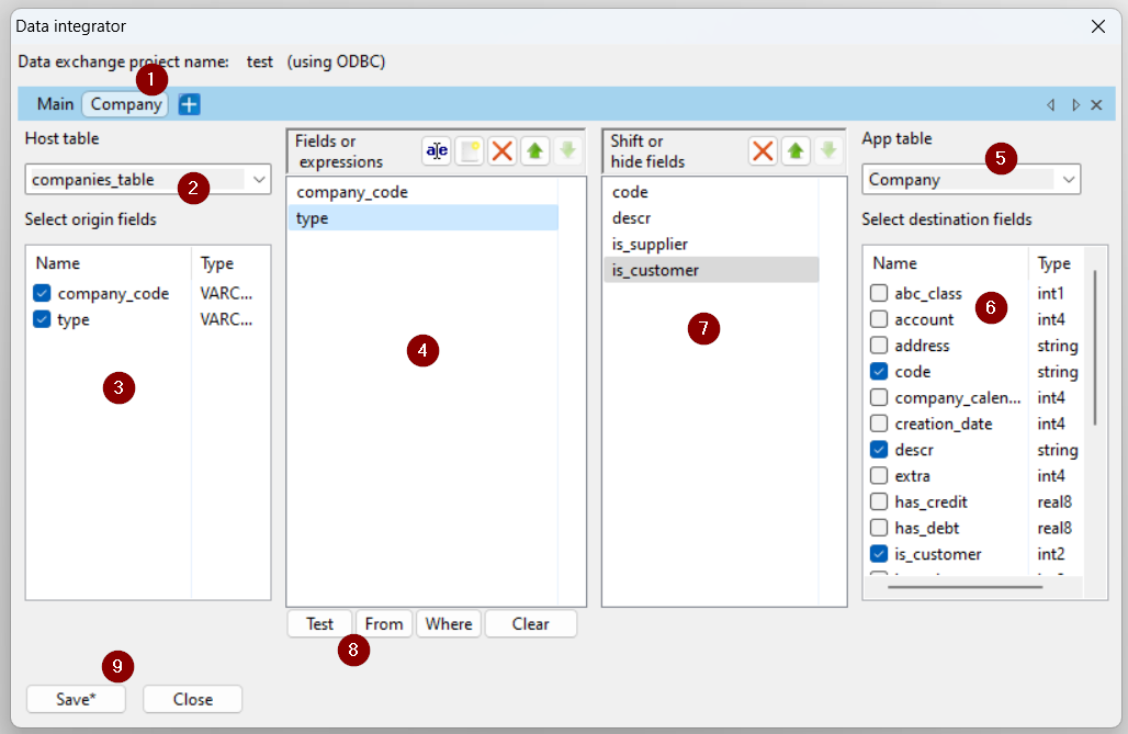
With the first click on the ‘+’ button, using the demo database, the following dialog box opens, structured as follows, with reference to the following image:

1. first of all, a page is created for mapping company registry data
2. select from the list the name of the data source table (host table) that contains the company data
3. once the name of the table has been selected, the list of fields that can be selected from this table is updated
4. the fields selected from the list in the previous point appear in this section; it is also possible to insert constants or SQL expressions
5. this list contains the names of the Apyesse database tables. Selecting a table updates the page name (1), however it can be modified with a right click on the tab, and the list of table fields is shown (6)
6. the list of table fields already opens with the main and mandatory fields selected, to facilitate the user’s operation
7. the selected Apyesse table fields are shown in this list and can be moved to those to which they should be mapped in the host table (4)
8. these buttons allow you to verify, test and modify the SQL statement that is generated by selecting the table and host fields
9. finally, after having mapped the various tables, click on ‘Save’ to save the data exchange project and to generate the Python script which will then be used to import data into APS

Once you have saved the data exchange project and created the data import Python script:

1. you select the script
2. its execution is launched

Once the data has been imported into Apyesse, it is possible to launch the calculation engines, consult the plan and make decisions. To do this, you can create custom views and window arrangements to operate in the most effective and efficient way

Configuring the graphical interface

This paragraph describes how to configure the graphic windows to facilitate data consultation and speed up decisions. In particular, a possible arrangement of windows is proposed for the analysis of purchase proposals.

Once the data has been imported, to generate reorder proposals for purchasing and production materials, the MRP must be performed by clicking on the button. After a few seconds, the order proposals will be present in the system.

At this point we want to create an arrangement of windows that allows us to easily identify the purchases to be made immediately and quickly understand the reasons why these purchases are needed.

Open the “Order Diagram” window from the following button on the toolbar and in the window that opens set the filters as shown in the figure:

Of all the orders and proposals present in the system we have narrowed our attention to the buy ones (B) with proposal status (0) and with an expected issue date within a week. At this point we want to associate this view with the pegging of the needs to have immediate evidence of the reasons that led the system to make these proposals to us.

As a first operation we click on the toolbar button so that the next windows that we open from contextual menus are connected to the initial one. Then by clicking with the right mouse button on the numerator of the proposal you choose “Windows” and then “Downstream Pert view” from the contextual menu.

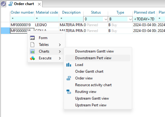
Another window will open next to the original window showing which orders material is required by our proposal. It is important to underline that these two windows are connected to each other: if in the first window you click on a cell of the proposal MF00000019, the second window updates and will show the network of assembly orders of this proposal.

We can now save this arrangement of windows to reuse it in subsequent planning sessions by operating as follows:

• click on the toolbar button
• in the dialog box, enter a name for the arrangement and possibly a group to which it belongs, as in the figure

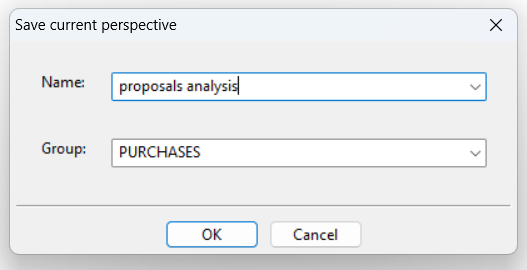
• after clicking on Ok, the new layout can be recalled from the layout menu as shown in the figure

Some notes:

• it is also possible to connect other windows to these and save the additions by clicking on “Save current layout” from the previous menu
• there is no limit to the number of arrangements that can be created
• Changes can be made to the created perspective to analyse, for example, the situation of a single supplier, in order to verify both new proposals and any need for reminders of orders already issued. To do this, simply change the filters in the first view

Please also note that different viewing options are available for each window, accessible via the button located in the top left corner of the window and which operates on the currently selected window.

One of the main distinctions to be aware of in supply chain planning is that between infinite capacity and finite capacity planning.

Infinite capacity planning:

• Create plans that respect the sequences of activities based on the product structure but without resolving the simultaneous commitment of production resources (machines, personnel)
• It is useful for evaluating production capacity adjustments required to meet customer delivery dates
• It is the only type of planning offered by the MRP modules of management systems (ERP), because it requires less processing complexity

On the other hand, finite capacity planning:

• Manages concurrent commitment of production resources and orders accordingly
• It is indispensable for creating feasible and credible plans, especially in the short term, when production capacity cannot be adjusted
• It is generally offered by APS systems, although with different levels of sophistication (some systems consider order components always available and simply sequence orders on a given resource)

This tutorial describes the data model and logic used by Apyesse to support infinite capacity and finite capacity planning.

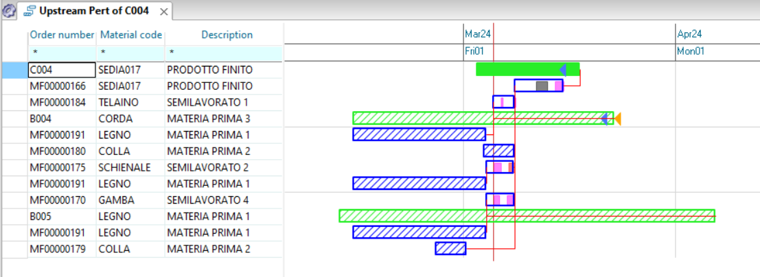
Infinite capacity planning is calculated by the MRP and CRP calculation engines, executed simultaneously by clicking on the button on the toolbar or by calling the corresponding function from a Python script. The result of this processing is exemplified in the following figure (limited to a single sales order for simplicity of presentation). In this figure:

• The solid bar represents a sales order: the left end corresponds to the order acquisition and the end of the bar corresponds to the delivery request date
• The bars below represent purchase orders (they are shaded) and production orders (they contain coloring bars that represent the processing phases). The colors of these rectangles are associated with the states: rectangles with a blue outline are proposed while the others are orders already issued or released
• The red lines connecting the various orders represent the combinations between commitments and expected arrivals
• Since the MRP calculation starts from the end date and proceeds with the calculations backwards in time (back scheduling), situations may arise in which the order proposals are in the past
• Furthermore, some orders already issued may have an arrival date later than one or more needs that they must satisfy (if a component is already available in stock, its orders are not displayed, please wait in this type of diagram

Since multiple independent needs (sales orders or forecasts) are simultaneously present within the plan, similar networks, orders and proposals are present to a large extent and, due to the fact that the processing is done at infinite capacity, situations can be created like the one in the figure for some resource (load greater than production capacity).

It is useful to note these situations because they allow you to evaluate whether to increase production capacity in periods of overload (for example by increasing shifts or using production capacity external to the company) but it is also important to be able to recalculate the plan in compliance with production capacity constraints where these cannot be removed.

If we look at the list of processing phases for center 001 above and the load profile is shown, we see that several are simultaneous, in finite capacity planning.

But if we launch the finite capacity scheduling execution we obtain their sequencing

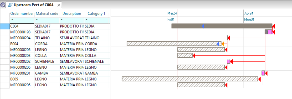
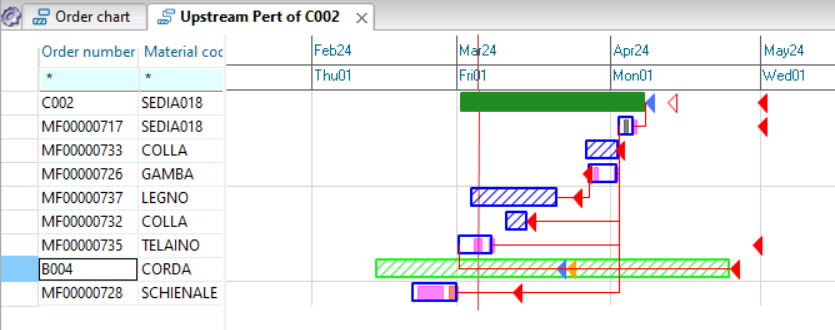
And this is also reflected in the dating of subsequent processing phases and other orders. This figure represents the lattice already seen but this time re-dated to finite capacity. In addition to resolving the constraint of the finite capacity of the machines, the constraint on the availability of materials is also respected, in fact:

• order MF00000072 cannot begin before the CORDA component has arrived with order B004
• purchase proposals in the past are rescheduled with the expected issue date equal to the current date and expected arrival date equal to today plus purchase lead time

Considering compliance with all these constraints, the simulated or scheduled delivery date for sales order C004 corresponds to the red triangle at the end of the corresponding rectangle. In addition to sales orders, the scheduled start and end dates are calculated for each type of order (purchase, production, transfer), for the processing phases and for warehouse commitments. These dates are managed in separate fields from those of infinite capacity planning, which therefore are not overwritten. In almost every graphic window of Apyesse it is possible to view the results of the calculation engines based on the scheduled dates (calculated by the scheduler) or with the so-called ‘planned’ dates (calculated by MRP or CRP or imported from ERP or other systems). In the graphic window above, the display of orders according to the scheduled dates is obtained by changing an option on the ‘window settings’ (menu accessible from the icon representing a gear at the top left) or, more easily, by clicking with the left mouse button mouse over the graphics area while holding down the ctrl key.

Even the load profiles, like the one previously represented, can be represented based on the dating of the scheduler and, in the case of the work center ‘001’ it appears to be as follows

Note that there are no longer any overloads: these have been ‘levelled’ to respect the production capacity constraint. In addition to the basic logic above, many options are available to drive the behavior of the finite capacity scheduler (FCS) calculation engine. These are the main ones.

Advance release

This item master parameter (‘advance_release_days’) expresses in working days the possible advance with which the scheduler can simulate the production or purchase of an order with respect to the planned dates (dates calculated with infinite capacity). Thanks to this parameter, any overloads can be resolved not only by delaying some processes but also by bringing them forward (the release advance is the maximum advance that can be attempted if resources and order components are available). THE fact that in the last figure the first week is saturated, while at infinite capacity it was not, is due to the management of a release advance greater than zero which allowed some processing to be brought forward

Work centers with finite and infinite capacity

In the work center registry, in addition to associating the calendar and shifts of the same, it is possible to differentiate which centers should be managed with finite capacity and which with infinite capacity using the ‘finite_capacity’ flag. It is also possible to define finite capacity management within a certain horizon via the ‘finite_capacity_horizon’ parameter (beyond this horizon the work center is scheduled at infinite capacity). This type of parameterization allows you to realistically manage real situations in which beyond a certain horizon the workload is low (customer orders for the period still have to be purchased) and it is possible to complete the management by valorising the queuing time of the fulfillment centre. I’m working to have a more plausible dating of the orders

Releasing components’ constraint

In some situations or in certain conditions of incomplete data it may be useful to consider only some orders or some materials as binding. To do this, these orders must be released by setting the ‘active’ flag to 0 in the “links between orders” table or perform the same action by selecting ‘execute’ and ‘release components’ from the contextual menu

Sequencing rules

In addition to allowing some processing phases to be brought forward to resolve overloads, the release advance serves to define a dynamic buffer of processing phases from which the scheduler can choose to optimize the processing sequences. With reference to the following figure, keep in mind that at any moment the scheduler looks ahead at a number of days equal to those defined on the material as the release advance (therefore generally different for different materials) and identifies a list of orders and their respective phases that can be scheduled. Among these, if you set sequencing rules and associate them with the processing phases of the attributes (‘status per processing cycle’ table), you can induce the scheduler and manage processing sequences in which the attributes are as homogeneous as possible or follow a certain desired sequence. Keep in mind that the greater the release advance (length of the blue arrow in the figure) the easier it becomes to find processing phases compatible with the one whose execution is being simulated (therefore the efficiency of the plan is increased) . However, there is a risk of anticipating convenient processes to the detriment of others that would need to be carried out to deliver soon-to-expire sales orders.

In the following figure, rules have been set to make it convenient to keep purple/pink phases together and green phases together.

For all these parameterizations it is advisable to check the Apyesse documentation in detail and use the demonstration archives to carry out tests and clarify any management doubts.

One of the most recurring planning tasks is estimating a delivery date for a new customer order. Where an APS is not used, we are often content to add a standard lead time by product type to the current date but these are very often very crude assessments, especially in times characterized by uncertainty in the supply of raw materials and components and with fickle demand .

Wanting to use Apyesse to support this type of process we have the following operations to perform:

• Open Apyesse and the current plan data model
• Enter the new independent requirement to be dated (or possibly multiple requirements if it is a request for several items)
• Launch the calculation in Apyesse
• Read the processing result

We describe the operation starting from the second point, taking the execution of the first for granted.

Enter the new independent requirements

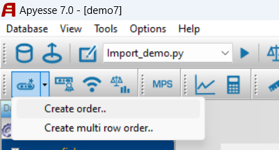
The Apyesse model is generally powered by other systems (ERP, MES) but can be integrated via script or via the user interface from other data. To calculate the delivery date of a customer order that has not yet been acquired, it is possible to simulate its acquisition by inserting it into Apyesse from the dialog box accessible from the “Create order” button on the toolbar and choosing “Create order..”.

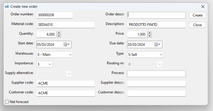
In the dialog box that opens, you essentially enter: the item, the quantity, the delivery request date and set other parameters as shown in the image (in general it is possible to simulate the insertion of orders of different types from those of sale). The order number is proposed directly by the system with the guarantee that it does not already exist (it is possible to change it as long as it is unique).

At the end of entering the new order with the “Create” button the calculation engines will be run to check whether the requested delivery date can be satisfied or whether the calculated one is different.

In addition to this entry method, it is possible to use another one, again from the user interface, which can be quicker in many cases. Suppose you have received from a colleague the requirements to be dated for a quote on a spreadsheet. It is possible to copy this data from the spreadsheet and insert it into Apyesse by simply pasting it, respecting some rather simple formatting and completeness rules. We proceed as follows:

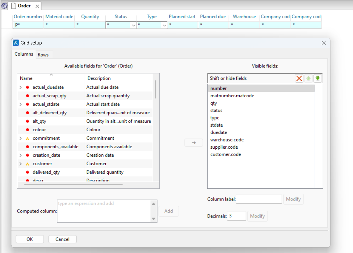
• We prepare a view in Apyesse into which we will paste the data from the spreadsheet, containing the following minimum data (first figure below)
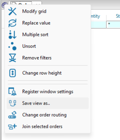
• Then you save this view for future reuse (second figure, “Save view as..”)

At this point you select the records from the spreadsheet without the column headers,

you press control+c, then you go to the view in Apyesse and press control+v.

At this point you can proceed with the calculation of the delivery date

Run the calculation engines

Now the two operations to carry out to calculate the delivery date of our requirements is to run MRP/CRP and scheduler in succession.

If the scheduled date does not satisfy us, we can investigate what points we can act on to improve the result. Generally both calculation engines run in a few seconds and the response on the delivery date can be provided to the sales colleague during a phone call or in any case in a very short time

The result of the processing

At the end of the calculation it can be verified that, given a requested date of February 28th, the system, with the capacity and availability constraints entered, has calculated a simulated delivery date of March 11th. Generally it is advisable to check how the result of the delivery date calculated by Apyesse has matured to make some evaluations.

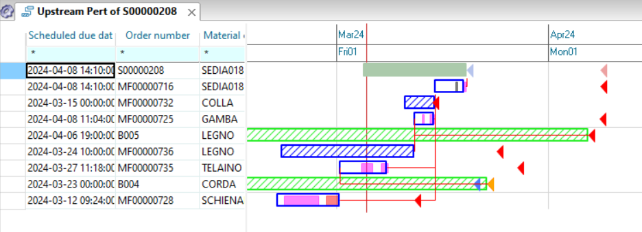
For example, critical issues such as the one in the figure may emerge, which demonstrate that a better date could be guaranteed to our customer if the supplier of order B004 was willing to bring forward the delivery of his goods. Other considerations could emerge from the analysis of load profiles, which could lead to varying the available production capacity to guarantee more favorable delivery dates

Furthermore, take into consideration the fact that to satisfy the order entered S00000009, the system may have distracted materials previously allocated from other customer orders to dedicate them to this new order. Where previously acquired sales orders are to be given priority in the allocation of material availability, it is possible to act in at least two different ways:

• configuring the MRP for special priorities, the subject of another section of the tutorials
• or by changing the status of the links between orders and those between needs and availability so that the MRP does not call them into question with the insertion of new needs

One of the main advantages of Apyesse is that it makes it possible to simulate new scenarios starting from the current state of production and the plan without requiring changes to the management system or particular IT skills to modify the data. In this tutorial we will see what are the various ways of varying the input data made available to the system in relation to the types of changes to the production structure that we want to simulate.

How to edit data

Editing from tabular grids

The content of Apyesse tables is represented using data grids and these are also present in numerous graphical views, such as for example in the order diagram.

To change data in a cell, simply double-click on a cell and type a new value or select one from the drop-down menu. You cannot modify values that correspond to key fields or key fields of linked tables.

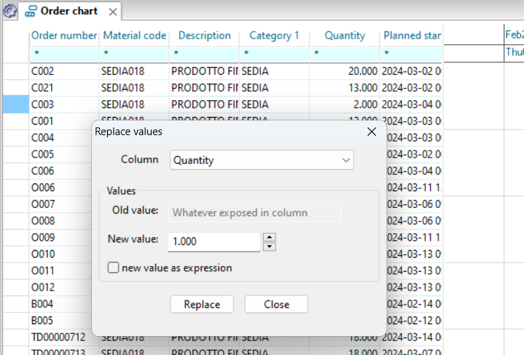
With data grids it is also possible to massively modify data. For example, if we want to change the quantity of orders in the grid we act as follows:

• click on a cell in the quantity column
• the view menu opens (gear icon) and select ‘Replace values’ (note that the column on which to perform the mass replacement can also be selected from here)

• at this point enter the new value under ‘New value’ and click on ‘Replace’

If you set the ‘new value as expression’ flag in the above dialog box, you can enter Python expressions in the cell next to ‘New Value’ to assign the new values. For example, the following expression tells the system to replace the current quantity with an increase of 20%.

current.qty*1.2

or, abbreviating ‘current’ (which represents the current record in the grid) with ‘c’:

c.qty*1.2

Keep in mind that with this mode only the records that appear in the data grid as a result of the filters are modified, not those that the filters hide.

Edit from tab

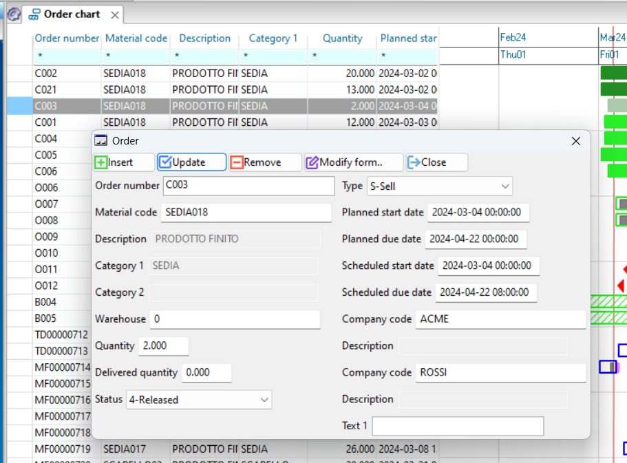
Another way to edit data is to do so using individual record tabs. This tab is opened by double clicking at the beginning of a line or from the contextual menu, selecting the ‘Tab’ item. In this case you change the value of a cell and then click on ‘Update’

Editing from script

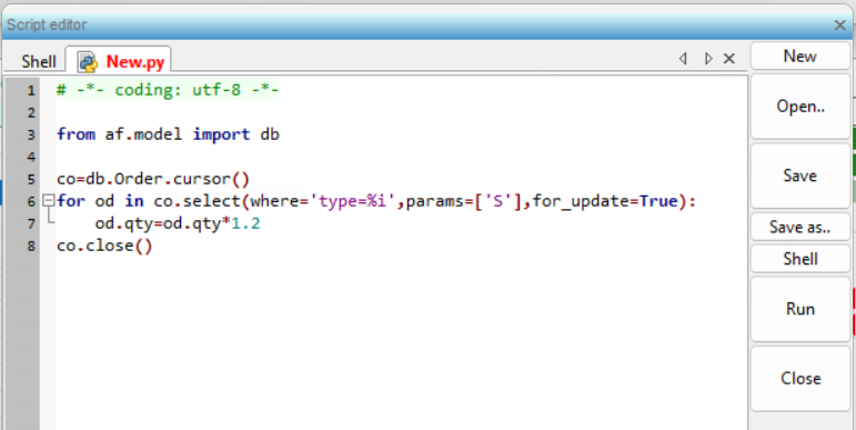
Editing data from scripts is the most flexible way, although it requires knowing a little Python. The methods of interaction with the Apyesse database are described in more detail in the Apyesse manual, while here the example of increasing the quantity of sales orders by 20% is given as an example.

Let’s now see which data makes sense to modify to evaluate new scenarios.

Changes to the material plan

Among the reasons why it may be useful to modify the material plan to simulate future situations and scenarios there may be, for example:

• evaluate the impact of sales increases on the production structure and cash flow (upward sales forecasts)
• evaluate the impact on deliveries to customers and on the production plan of extensions of supplier delivery lead times
• evaluate the impact on inventory levels of changes to material safety stocks

To increase the values of the forecast requirements it may be useful to operate as previously described regarding the mass replacements of values in the data grid. This type of data intervention presupposes that the forecast records are already present in Apyesse. If they are not, it is possible to load them from scripts from different types of data sources, or from a spreadsheet with a copy and paste as described in the tutorial regarding data exchange with Excel. A similar situation applies to safety stocks: if the safety stock records are already loaded in the ‘Safety stock’ table then the modification of the values can be done with a mass replacement, otherwise the records must first be inserted into the database.

Regarding the change in supplier delivery times:

• by changing the lead time on the item master data, the proposals generated by the MRP are affected by the change
• If you also want to change the delivery dates of orders already issued to suppliers (for example due to problems with the supplier), you can change the delivery dates (‘duedate’) even massively as follows (10 days is an example):

c.duedate+datetime.timedelta(days=10)

also in this case a Python expression is used to perform more complex substitutions than a single value.

Changes to the capacity and load plan

Other simulations may concern the capacity and load plan, for example to evaluate:

• impact on delivery dates to customers resulting from additional shifts on work centers
• consequences on workloads resulting from increases in sales forecasts
• impact on delivery dates to customers of prolonged downtime of some machines

We have already described in the previous point how to simulate the change in forecast needs. The impact these have on workloads is visible after the MRP/CRP is launched by clicking on the button.

As regards changes to production capacity linked to shifts and calendars, we act as follows.

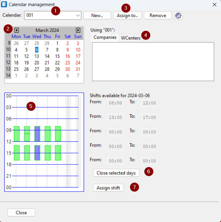
Each work center is associated, where mandatory, with a calendar with shifts. The calendar associated with one (or more) work centers is visible on the work center card itself or in the data grids. Once you know the name of the calendar, you can recall it from the dialog box that opens from the toolbar button.

In this dialog box we find:

1. the menu to select the calendar to consult or modify
2. the display of the days for which the configured shifts are to be examined
3. some keys to create a new calendar, assign an existing one to work centers or suppliers, delete them from the database and a key to change the display settings of the dialog box
4. some cards to check which work centers and companies the calendar is associated with
5. the detail of the active shifts for the day selected in the element referred to in point 2
6. a button to decide to remove shifts from the selected day or days out of 2
7. a button to assign new shifts to the day or days selected in 2 (clicking on it opens a window with the selectable shifts)

Once the changes have been made, the production capacity is modified but it is necessary to relaunch the MRP/CRP and the scheduler to have the system re-evaluate the possible delivery dates for customer orders.

Changes to the scheduled plan

Given a certain material plan and the capacity and workload plan also fixed, the simulations that can be performed with the calculations and constraints of the scheduler as reference can be, for example, the following:

• release production orders from certain components coming from suppliers or other departments to clarify how much delivery dates to customers depend on internal or external bottlenecks
• evaluate the impact of different scheduling strategies on production efficiency (less tooling), meeting delivery dates and WIP

To release components, you can act selectively on the Order Links table to deactivate the appropriate records, thus relaxing the precedence constraint on some orders. In the second case the parameters to be modified can be multiple and among these:

• the order release advance, i.e. the horizon in working days used by the scheduler, in a differentiated way for various materials, to determine the buffer of orders from which to choose the next one to execute. Generally, the higher this parameter is, the more efficient the calculated sequences are in terms of optimizing the setup but at the probable expense of punctuality of deliveries.
• the attributes to maintain continuity with production changes (same paint or same machine tooling, etc.), managed in the State tables for processing cycle (see the Apyesse documentation for further details.

 

Monte Carlo simulation

The topic covered in this paragraph is certainly at an advanced level compared to the simulations described in the previous paragraphs and deserves a more detailed introduction.

When you create a production and purchasing plan on a certain date, deterministic assumptions are made about many events in the plan. For example: we plan to start a certain production order in 5 days because on that date we will have the raw material ordered from the supplier and which, for his confirmation, will arrive, for example, in 3 days. In reality the production order can start in five days if:

• the supplier is reliable and will deliver the order to us on time
• production on the same machine in the next 5 days will not have significant variations, such as to have to delay the production of our order
• the availability of the machine is guaranteed (no breakdowns or absenteeism)
• there are no urgent reasons (new priority customer orders) to change the plan established today

In reality there are always some disturbances, to varying degrees depending on how predictable our and our suppliers’ production processes are. What is certainly certain are the decisions to be implemented immediately, what in jargon are called ‘first period decisions’. How can we be reasonably certain that, in the face of all the disruptions that our production system may have over time, we will be able to satisfy the market in an adequate and sufficiently predictable way? To make this type of assessment, Monte Carlo simulations can be used, i.e. a type of simulation in which perturbations are introduced to expected events to understand whether the company’s performance is sufficiently protected from events that are not entirely controllable. The general scheme for running a Monte Carlo simulation is the following (can be achieved using Python scripts):

• we start with the production plan calculated as of today with the current data and release some production and purchase orders (those needed immediately)
• then the progression of time is simulated (for example the current date is increased by one day) and changes are made to the data of this type:
  • purchase orders that were supposed to arrive today are closed and the inventory is increased accordingly. Or you choose to pay only some orders and send others late in delivery to simulate the unreliability of deliveries
  • new customer orders are entered into the system
  • processing phases that should be closed are closed and some are left open among those that should have been carried out with the date change
  • some expired or expiring customer orders are closed to simulate shipping
• the calculation engines are launched to create the new plan and we start again from the first point

By carrying out this cycle for a number of times (days) equal to a few weeks, it is possible to better evaluate the expected delivery date for a customer order or, more generally, the level of service to the market. If we have a particularly problematic supplier in terms of reliability of delivery dates, we can simulate the impact of this behavior on the performance of our company and compare it (simulating it) with that of any more reliable alternative supplier

How to compare the results of different parameterizations

Unlike other Paneido solutions, Apyesse does not include a KPI dashboard per scenario, so it is up to the user to record the monitored outputs at each parameter change and subsequent recalculation (manually or via script). For example, to compare the impact on the simulated (scheduled) delivery dates of two different parameterizations, you can proceed as follows:

• the calculation engines are launched and in particular the scheduler (FCS) to have the system calculate the scheduled dates, displayed with red triangles next to each order
• then select the orders (all or part) and from the contextual menu choose ‘Execute’ -> ‘Save scheduled dates as previous’. This operation copies the values of the ‘s_duedate’ field of the orders into the ‘previous_s_duedate’ field of the same orders (this operation can also be performed by script)
• then you modify some data and relaunch the MRP and scheduler to have the system calculate new scheduled dates

Visually it is possible to compare the new dates with the previous ones as in the figure where you can see that for order C004 the new date (full red triangle) is later than the previous scheduled date (white triangle with red outline)

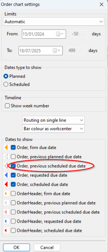
To view the red triangles with white interior (previous scheduled dates), which by default are not displayed, click on the gear icon in the top left corner and select ‘Change settings’. In the dialog box that appears opens and select the item ‘Order, previous scheduled end date’ as shown in the figure

For completeness: to move from the first scenario to the second, the modification that has been made to the data is the postponement of the delivery of the purchase order B004 obtained by dragging the right side of the rectangle in the graphic part to the right with the mouse (this operation is equivalent to change the scheduled end date of the or1der from the form or from the data grid or from the script)

One of the main advantages of Apyesse is that it allows you to run simulations locally without requiring changes to input data shared with other systems. Among the simulations supported by Apyesse is the cash flow simulation and is a functionality linked to the calculations performed by the finite capacity scheduling engine.

Required data

The cash flow simulation is grafted onto the data model already created to support planning and scheduling processes. To this must be added:

• enabling the recording of simulated cash movements
• the payment policies of customers and suppliers
• cash flow contributions not managed directly by Apyesse

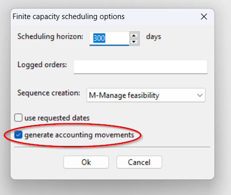
As regards the first point, it is necessary to set the ‘generate financial movements’ option in the FCS (Finite Capacity Scheduler) Options, as in the figure

Customer and supplier payment policies

For each company listed in the Company table it is possible to associate a payment policy as follows:

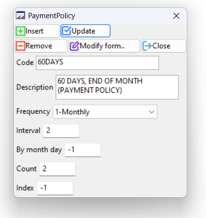
• a record is defined in the Payment Policy table where the identifying name, any description and the default extension are indicated. For example, to define “60 days end of month” you set the parameters as shown in the figure. The deadline creation logic is based on recurrences: it indicates the last day of the month (-1) of a succession of two consecutive months (see the Apyesse manual for a more detailed description of the parameters)

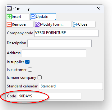
• this policy is associated with the supplier or customer companies with which it is agreed in the ‘paymentpolicy.code’ field, as in the figure

the one described is the basic modeling. It is also possible to associate each company with an account (and its account type) in order to further detail the various contributions to the cash flow.

Other contributions to cash flow

Apyesse’s distinctive contribution to cash flow simulation is the ability to model the contributions of customer and supplier payments by linking them to the events of the production and purchasing plan, with its constraints. To have a complete cash flow situation, Apyesse allows you to manage other contributions in two ways:

• importing them from outside or in any case forcing them into a Python script and populating the ‘Financial movements’ table
• or by defining the frequency of generation of recurring contributions (monthly or with other periodicity) in the ‘Financial movement generator’ table

Creation of scenarios

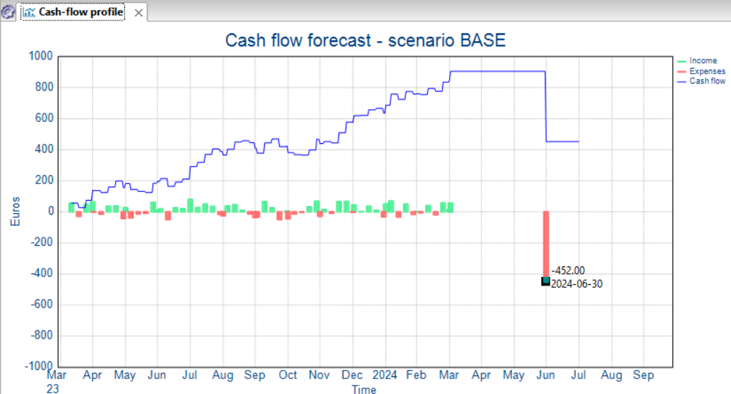
Starting from the planning and scheduling model and setting the additional parameters as previously described, it is sufficient to run MRP/CRP and scheduler to have a first cash flow profile, assigned to the default ‘BASE’ scenario. The various contributions of this profile are contained in the ‘Financial movements’ table while its graphic representation is obtained by clicking on the following toolbar button. The result obtained is of this type:

To evaluate one or more alternative scenarios, proceed as follows:

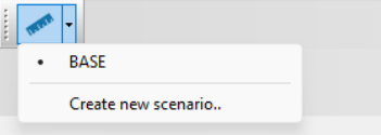
• a new scenario is defined by clicking on the following toolbar button and choosing “Create new scenario..”

• then you modify the plan data: for example by importing sales forecasts or modifying the arrival dates of purchases or the payment terms of customers and suppliers or the parameters for reordering materials or the production capacity
• at this point the MRP/CRP and the scheduler are relaunched and the new profile is obtained, displayed like the previous one but taking advantage of the fact that the current scenario is now ‘NEW’

In the ‘Financial movements’ table we currently find:

• the movements common to both scenarios (they do not have the reference to the completed scenario)
• those specific to ‘BASIC’ and those to ‘NEW’

Sharing results

If the company already has dashboards for consulting the forecast cash flow profile (on business intelligence systems or specific applications), it is possible to export the contributions calculated by the system from Apyesse in a similar way to how the data relating to planning and production and purchasing scheduling: a Python script is written and the data is transferred using protocols such as ODBC or REST or by generating text files (or csv or xlsx) to import into the other system.

The data exchange between Apyesse and spreadsheets offers great flexibility for making Apyesse results usable for other users and for feeding the input data. In particular, when using Excel as a data source for Apyesse, you can obtain useful results in a short time.

How to use Excel to feed the Apyesse database

The two main methods that can be exploited are:

• Copy tabular data from Excel and paste it into an Apyesse data grid
• Import data from Excel into Apyesse using a Python script

Copy and paste from Excel

This method was also illustrated in the tutorial regarding the dating of new orders with Apyesse. We proceed as follows:

• prepare the data in tabular form in Excel to paste into Apyesse
• a given grid is prepared in Apyesse with the same columns as the Excel sheet, respecting some constraints on the minimum data provided by the various tables
• select the cells from Excel, excluding the column headers and copy the data (ctrl+c)
• then click on the data destination area in Apyesse and press ctrl-v

If there are incompatibilities in the data format, warning messages will be issued by the application. In particular, the following aspects must be kept in mind:

• some fields in the various tables are references and must be respected. For example, if you paste data into the Order table, the item codes to which the new orders are addressed must have been previously inserted in the Material table (imported from script or pasted)
• various data formats are automatically recognized, in particular the separators between year, month, day
• in the Material table the mandatory fields are the item code and that of the main supplier (which, being a reference to the company database, must have been previously loaded into this table)
• in the Stock table the lot code (possibly empty), the item code and warehouse code are mandatory
• in the Order table the following must be specified:
  • record identification numerator (it is sufficient to be a progressive number whose value is not yet present in the database)
  • article code (must refer to an article already present in the database)
  • warehouse code (must refer to a warehouse already present in the database)
  • quantity
  • type of order (S if it concerns independent requirements such as customer orders or forecasts)
  • scheduled start date (the current date)
  • scheduled finish date (your target date for delivery)
  • supplier code (must refer to a company already present in the database)
  • customer code (must refer to a company already present in the database)
  • order status (generally okay 3)

Importing data from Excel using Python scripts

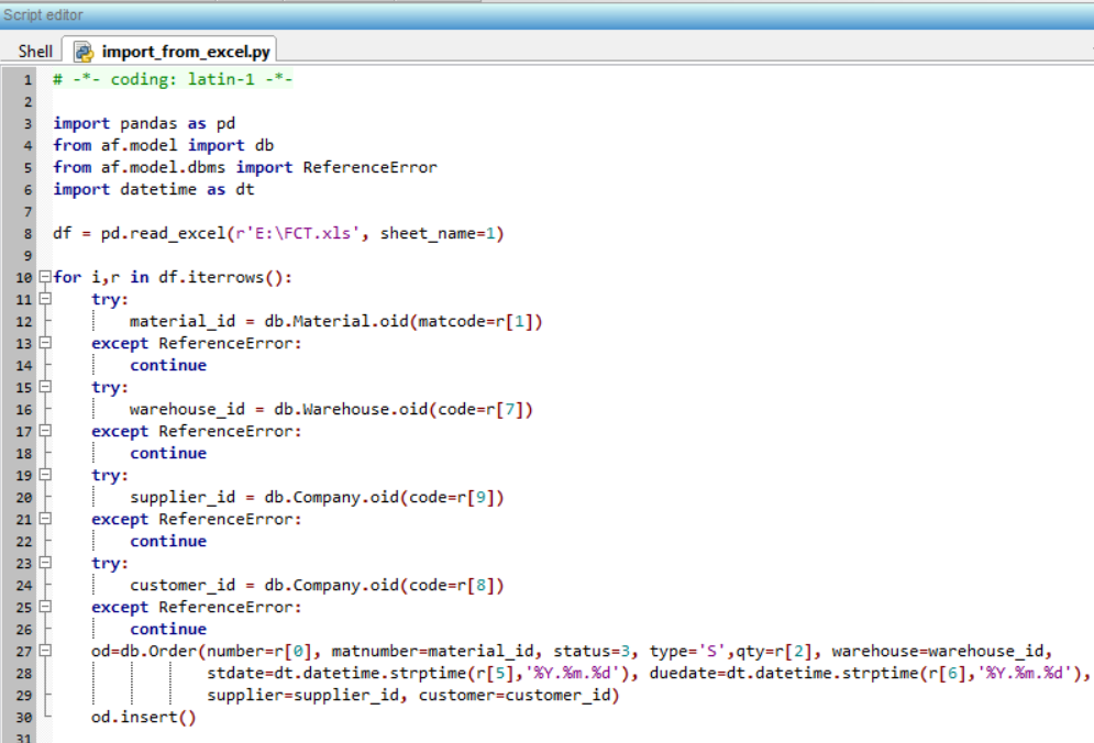
Apyesse includes several libraries that can be used to read data from Excel. The main ones are xlrd, openpyxl, pandas. Here is an example script that uses pandas to read data in a dataframe and then pass it into the Apyesse Order table.

This is the sheet that reports the data (it is the second sheet of the file).

And this is the script that imports data from the spreadsheet into Apyesse. As regards the reference type fields (warehouse, item, supplier, customer), it is checked whether the corresponding data is already present in the respective table, otherwise the Excel sheet row is skipped.

How to transfer data from Apyesse to Excel

Also for passing data from Apyesse to Excel it is possible to use copy and paste or a Python script. Furthermore, since it is possible to create pivot tables with Apyesse grid data, it is also possible to export these pivot tables to a spreadsheet.

Copy from Apyesse and paste into Excel

After opening the data grid or a graphic window containing the grid, select all the records by clicking with the left mouse button in the rectangle at the top left of the grid (the rows of the grid turn blue).

Then, by simultaneously holding down the ctrl key and the left mouse button, you drag the selection into the open spreadsheet. Alternatively, press ctrl+c in Apyesse and then ctrl+v in Excel.

If filters or sorting have been set in the data grid, these settings are also respected in the data passed to Excel. Same thing for any calculated columns (i.e. result of an expression) present in the data grid.

Export data from Apyesse to Excel using a Python script

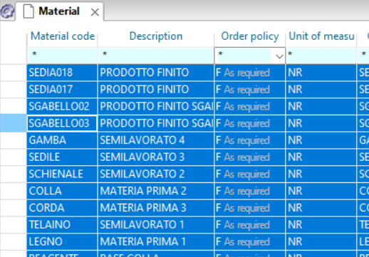
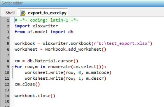
The following script exports Apyesse item master data to an Excel file using the xlsxwriter library, also included in Apyesse. The same operation is also possible with pandas or xlwt, for example. Please refer to the documentation for these libraries for formatting instructions. To retrieve data from the Apyesse database you need to open a cursor in the corresponding table and then run a query. In this case we operate directly on the database, therefore without referring to the content and filters of a specific data grid.

Saving a pivot table created with Apyesse in Excel

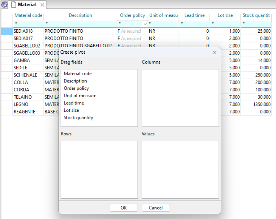
In Apyesse it is possible to create pivot tables starting from a data grid. To do this, click with the right mouse button on the rectangle at the top left of the data grid and operate in the dialog box that opens to set the pivot.

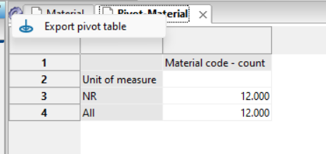
Once finished, click on ok and a new data grid containing the pivot will open. At this point you can save the pivot in Excel (without the structure) by clicking on the gear at the top left and choosing “Export pivot table”.

The basic logic of each MRP module and also that of Apyesse provides that the needs of a given material are served in ascending order of date.

However, this means that, in the absence of other mechanisms, an order that today commits a stock of a given material may have this allocation subtracted from a new order just entered into the system with an earlier commitment date. This is a situation that disorientates the planner and does not allow him to fix the decisions he has made. To overcome situations of this type, in Apyesse it is possible to define that:

• for certain items, along a horizon defined per item, the allocation of availability is not done by commitment date but: up to a certain date according to a customizable sequence of commitments and beyond by date
• the special ordering of commitments within the defined horizon can follow various criteria in cascade

Thanks to this it is possible, for example:

• ensure that a released production order preserves the allocation of component stocks even in the presence of a new order proposal that commits the same component on an earlier date
• give higher priority to customer orders for spare parts than those for finished products
• make certain types of customers priorities
• favor the delivery of small quantities to several customers rather than a large quantity to a single customer
• propagate the importance of the customer order served also to the lower levels of the bill of materials
• favor the satisfaction of a commercial requirement (customer order) over a sales forecast

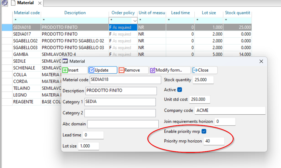
Going into more detail, on the item master there are two parameters linked to the management of the MRP for special priorities:

• the ‘enable priority mrp’ flag which enables management
• ‘priority_mrp_horizon’ which establishes the horizon on which to use the special rules

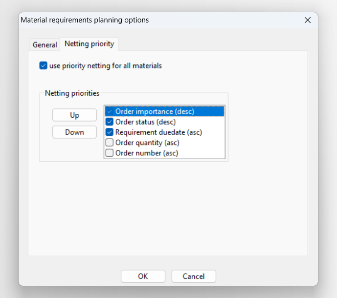
In the MRP options you select and order the rules to be used along the horizon managed for special priorities

In particular, the ‘importance’ parameter managed on orders and indirectly on their requirements proves to be particularly powerful because it can be valorised during data import in a differentiated way on customer orders or on various types of production orders. Furthermore, the importance can then be propagated from finished product orders towards semi-finished products and proposals and purchase orders by setting the last parameter of this MRP options window

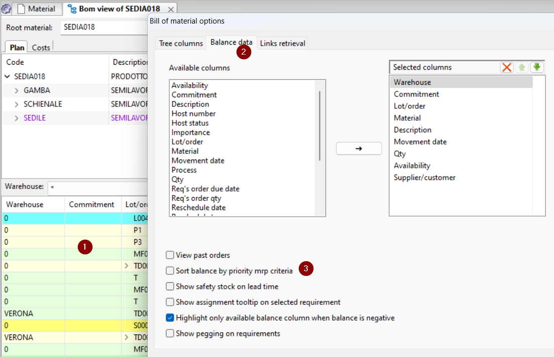
Once the parameterization has been completed and Apyesse carries out the calculations according to the settings, it can sometimes be difficult to detect the calculation logic from the application’s graphic windows if they order the data by date (and not by order of satisfaction of needs) and if the netting horizon for special priorities is quite high (approximately more than two weeks). In these cases it may be useful to consult the requirements balancing profile, present in the lower part of the “Bill of materials” and “Where is it used” windows, having selected the “Order item balance according to MRP criteria for special priorities” option.

Please note that Apyesse offers various other possibilities for configuring the combinations between availability and needs. The two main areas of functionality in this sense concern:

• the management of the MRP by commitment/contract together with that by requirement (i.e. without order references on availability and requirements)
• the management of availability transfer proposals between warehouses, in the context of which it is defined which commitments can be netted for certain warehouses and under what conditions

For further information on these areas, please refer to the online documentation of the Apyesse application

Apyesse stands out from many advanced planning systems because in addition to being structured to manage the most usual planning activities (order release, missing analysis, etc.) it has the flexibility and functionality needed for high-level checks and simulations. This tutorial describes how to evaluate inventory that is in excess of the current production plan or other scenarios.

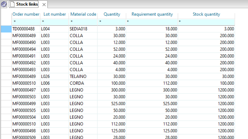
First of all, keep in mind that the MRP procedure with active (preset) link generation provides as output the links between needs and availability at all levels. In particular, the links between stocks of various materials and related commitments (whether actual or forecast) are written in the table. The following image shows the contents of the “Inventory-requirements links” tables for a demonstration data archive. The identification number of the binding order appears in the first column (be it a transfer, sales or production order). The quantities that appear in the fourth column do not represent the quantity of stock, nor that of the requirement, but the quantity of the stock record assigned to that requirement. So in the first case the transfer order ‘TD00000488’ commits 18 pieces of SEDIA018. Of these 18 pieces, 3 is allocated to stock lot L004 which has 3.

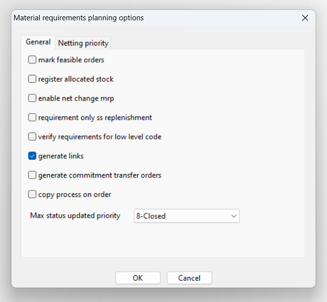
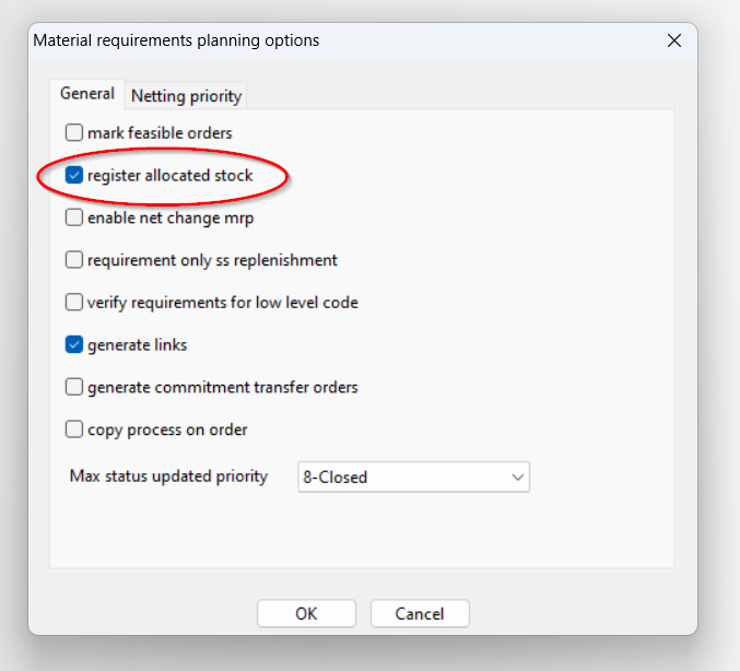
By enabling the flag in the figure on the MRP options, Apyesse records and sums all these allocations in the ‘allocated_qty’ field of the ‘Inventory’ table and this is the basis for evaluating the value of excess inventory.

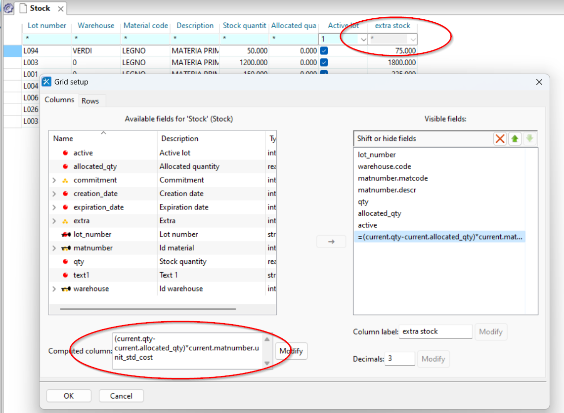
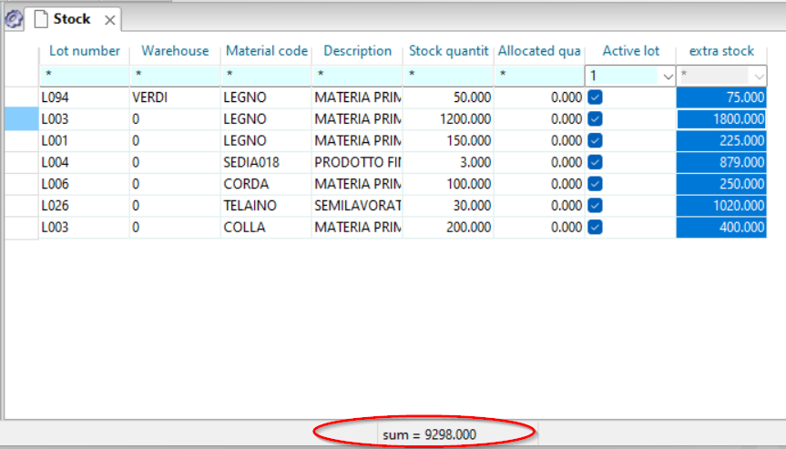
Now, having already run the MRP, we open the ‘Inventory’ table and create a view like the one in the figure, where we have inserted an expression in a column that represents the difference between inventory and allocated inventory (the result is the free inventory) multiplied by the value of the material.

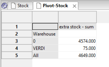
At this point if we select the column containing the expression and we press F6 to obtain the total free stock value on the status bar. Alternatively, you can create a pivot table by item category or by warehouse to better see how excess inventory is distributed.

It is possible to evaluate this excess inventory in the presence of different sets of needs. For example, different sales budget hypotheses could be loaded into Apyesse and for each one, by running the MRP, it is possible to check which items are at greatest risk of obsolescence.

Other graphical options for evaluating excess inventory are also available in other Paneido planning systems